Blog post for Week 3 of Machine Learning for Data Analysis (Coursera)
What is Lasso Regression Analysis?
Lasso regression analysis is a shrinkage and variable selection method for linear regression models. The goal of lasso regression is to obtain the subset of predictors that minimizes prediction error for a quantitative response variable. The lasso does this by imposing a constraint on the model parameters that causes regression coefficients for some variables to shrink toward zero. Variables with a regression coefficient equal to zero after the shrinkage process are excluded from the model. Variables with non-zero regression coefficients variables are most strongly associated with the response variable. Explanatory variables can be either quantitative, categorical or both.
Analysis Process
- Selecting a dataset: The chosen data set was the forest fires from the UCI Machine Learning Repository, where the aim is to predict the burned area of forest fires, in the northeast region of Portugal, by using meteorological and other data. The data set consists of 517 observations and 12 predictor variables and 1 response of the total area burned from the forest fire. There are no missing values.
[Cortez and Morais, 2007] P. Cortez and A. Morais. A Data Mining Approach to Predict Forest Fires using Meteorological Data. In J. Neves, M. F. Santos and J. Machado Eds., New Trends in Artificial Intelligence, Proceedings of the 13th EPIA 2007 - Portuguese Conference on Artificial Intelligence, December, Guimarães, Portugal, pp. 512-523, 2007. APPIA, ISBN-13 978-989-95618-0-9. Available at: Web Link.
- Data cleaning & pre-processing in R: I will eventually learn to use the urllib package for running this entire analysis in python, but as a scrappy data scientist I will use the best tools at my disposal, which include R programming. In R I read in the url to obtain the csv and constructed design matrix (aka a model matrix) which imputes binary responses for categorical variables. I wrote a new csv file to my working directory.
R code:
library(RCurl)
url = getURL("http://archive.ics.uci.edu/ml/machine-learning-databases/forest-fires/forestfires.csv")
forest_fires <- read.csv(text = url)
head(forest_fires)
# get a model matrix
ff_clean = model.matrix(~.,  data=forest_fires)
ff_clean = as.data.frame(ff_clean)
# write the csv file to my coursera folder
library(readr)
write_csv(x=ff_clean, path="C:/Users/JD87417/Desktop/python work/Coursera/forest_fires.csv")
# get column print out for python (line 19)
library(pystr)
cols = colnames(ff_clean)
dput(pystr_upper(cols))
- Python Methodology: In python I used pandas, numpy, matplotlib, and sklearn. The cleaned dataset was read in and column names were made uppercase and missing values removed (not necessary for this dataset). The predictor variables were selected as a new data frame and the target variable of
areawas specified. The predictors were then standardized (or scaled) so that the rows-columns would have a mean = 0 and a standard deviation = 1. This ensures that variables on different scales (i.e. ounce versus pounds) contribute equally to the analysis. TheLassoLarsCVfunction was run on the training set and the produced the regression coefficients which indicates the strongest variable(s) correlated with the response.
Results
A lasso regression was completed for the forest fires dataset to identify a subset of variables from a set of 12 categorical and numerical predictor variables that best predicted a quantitative response variable measuring the area burning by forest fires in the northeast region of Portugal. The data were randomly split into a train and test dataset that included 70% of the observations and test set that included 30%. The least angle regression algorithm with folds equal to 10 (5 or 10 are optimal number of folds) for cross validation was used to estimate the lasso regression model in the training set and the model was validated using the test set, to prevent over fitting the model. The change in the cross validation average (MSE) at each step was used to identify the best subset of predictor variables which were:
- DAYSAT: Day of the week, Saturday
- TEMP: temperature in Celsius degrees: 2.2 to 33.30
- X: x-axis spatial coordinate within the Montesinho park map: 1 to 9
The 3 most important predictors have non-zero coefficients and therefore can be the best subset to predict the amount of area burned by forest fires. These variables make sense when evaluating the highest probable chance for forest fire would be high TEMP, and DAYSAT equating to populous park attendance on the weekend which could be started by camping activity. The X variable is a bit tricky to interpret but I’m going to infer that the spatial coordinate is related to forest fire frequency and occurrence. This analysis reduces the variables needed to predict the area burned by forest fires in Portugal and therefore reduces the model complexity for a parsimonious model.
Additional Documents
- Jupyter Notebook: https://github.com/jasdumas/jasdumas.github.io/blob/master/post_data/Lasso_regression_forestfires.ipynb
- Python Code: https://github.com/jasdumas/jasdumas.github.io/blob/master/post_data/lasso_forerst_fires.py
- R code: https://github.com/jasdumas/jasdumas.github.io/blob/master/post_data/python_forestfire_clean.R
- Final Excel csv: https://github.com/jasdumas/jasdumas.github.io/blob/master/post_data/forest_fires.csv
Python code
#from pandas import Series, DataFrame
import pandas as pd
import numpy as np
import matplotlib.pylab as plt
from sklearn.cross_validation import train_test_split
from sklearn.linear_model import LassoLarsCV
#Load the dataset
data = pd.read_csv("C:/Users/JD87417/Desktop/python work/Coursera/forest_fires.csv")
#upper-case all DataFrame column names
data.columns = map(str.upper, data.columns)
# Data Management - remove missing values
data_clean = data.dropna()
#select predictor variables and target variable as separate data sets
predvar= data_clean[["X", "Y", "MONTHAUG", "MONTHDEC", "MONTHFEB",
"MONTHJAN", "MONTHJUL", "MONTHJUN", "MONTHMAR", "MONTHMAY", "MONTHNOV",
"MONTHOCT", "MONTHSEP", "DAYMON", "DAYSAT", "DAYSUN", "DAYTHU",
"DAYTUE", "DAYWED", "FFMC", "DMC", "DC", "ISI", "TEMP", "RH",
"WIND", "RAIN"]]
target = data_clean.AREA
# standardize predictors to have mean=0 and sd=1
predictors=predvar.copy()
from sklearn import preprocessing
predictors['X']=preprocessing.scale(predictors['X'].astype('float64'))
predictors['Y']=preprocessing.scale(predictors['Y'].astype('float64'))
predictors['MONTHAUG']=preprocessing.scale(predictors['MONTHAUG'].astype('float64'))
predictors['MONTHDEC']=preprocessing.scale(predictors['MONTHDEC'].astype('float64'))
predictors['MONTHFEB']=preprocessing.scale(predictors['MONTHFEB'].astype('float64'))
predictors['MONTHJAN']=preprocessing.scale(predictors['MONTHJAN'].astype('float64'))
predictors['MONTHJUL']=preprocessing.scale(predictors['MONTHJUL'].astype('float64'))
predictors['MONTHJUN']=preprocessing.scale(predictors['MONTHJUN'].astype('float64'))
predictors['MONTHMAR']=preprocessing.scale(predictors['MONTHMAR'].astype('float64'))
predictors['MONTHMAY']=preprocessing.scale(predictors['MONTHMAY'].astype('float64'))
predictors['MONTHNOV']=preprocessing.scale(predictors['MONTHNOV'].astype('float64'))
predictors['MONTHOCT']=preprocessing.scale(predictors['MONTHOCT'].astype('float64'))
predictors['MONTHSEP']=preprocessing.scale(predictors['MONTHSEP'].astype('float64'))
predictors['DAYMON']=preprocessing.scale(predictors['DAYMON'].astype('float64'))
predictors['DAYSAT']=preprocessing.scale(predictors['DAYSAT'].astype('float64'))
predictors['DAYSUN']=preprocessing.scale(predictors['DAYSUN'].astype('float64'))
predictors['DAYTHU']=preprocessing.scale(predictors['DAYTHU'].astype('float64'))
predictors['DAYTUE']=preprocessing.scale(predictors['DAYTUE'].astype('float64'))
predictors['DAYWED']=preprocessing.scale(predictors['DAYWED'].astype('float64'))
predictors['FFMC']=preprocessing.scale(predictors['FFMC'].astype('float64'))
predictors['DMC']=preprocessing.scale(predictors['DMC'].astype('float64'))
predictors['DC']=preprocessing.scale(predictors['DC'].astype('float64'))
predictors['ISI']=preprocessing.scale(predictors['ISI'].astype('float64'))
predictors['TEMP']=preprocessing.scale(predictors['TEMP'].astype('float64'))
predictors['RH']=preprocessing.scale(predictors['RH'].astype('float64'))
predictors['WIND']=preprocessing.scale(predictors['WIND'].astype('float64'))
predictors['RAIN']=preprocessing.scale(predictors['RAIN'].astype('float64'))
# split data into train and test sets
pred_train, pred_test, tar_train, tar_test = train_test_split(predictors, target,
test_size=.3, random_state=123)
# specify the lasso regression model
model=LassoLarsCV(cv=10, precompute=False).fit(pred_train,tar_train)
# print variable names and regression coefficients
dict(zip(predictors.columns, model.coef_))
# plot coefficient progression
m_log_alphas = -np.log10(model.alphas_)
ax = plt.gca()
plt.plot(m_log_alphas, model.coef_path_.T)
plt.axvline(-np.log10(model.alpha_), linestyle='--', color='k',
label='alpha CV')
plt.ylabel('Regression Coefficients')
plt.xlabel('-log(alpha)')
plt.title('Regression Coefficients Progression for Lasso Paths')
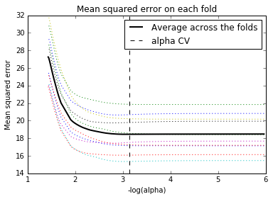
# plot mean square error for each fold
m_log_alphascv = -np.log10(model.cv_alphas_)
plt.figure()
plt.plot(m_log_alphascv, model.cv_mse_path_, ':')
plt.plot(m_log_alphascv, model.cv_mse_path_.mean(axis=-1), 'k',
label='Average across the folds', linewidth=2)
plt.axvline(-np.log10(model.alpha_), linestyle='--', color='k',
label='alpha CV')
plt.legend()
plt.xlabel('-log(alpha)')
plt.ylabel('Mean squared error')
plt.title('Mean squared error on each fold')
# MSE from training and test data
from sklearn.metrics import mean_squared_error
train_error = mean_squared_error(tar_train, model.predict(pred_train))
test_error = mean_squared_error(tar_test, model.predict(pred_test))
print ('training data MSE')
print(train_error)
print ('test data MSE')
print(test_error)
# R-square from training and test data
rsquared_train=model.score(pred_train,tar_train)
rsquared_test=model.score(pred_test,tar_test)
print ('training data R-square')
print(rsquared_train)
print ('test data R-square')
print(rsquared_test)